Video Prediction using ConvLSTM Autoencoder (PyTorch)
In this guide, I will show you how to code a ConvLSTM autoencoder (seq2seq) model for frame prediction using the MovingMNIST dataset. This framework can easily be extended for any other dataset as long as it complies with the standard pytorch Dataset configuration.
Before starting, we will briefly outline the libraries we are using:
python=3.6.8
torch=1.1.0
torchvision=0.3.0
pytorch-lightning=0.7.1
matplotlib=3.1.3
tensorboard=1.15.0a20190708
1: Dataloader
Download the dataloader script from the following repo tychovdo/MovingMNIST.
This dataset was originally developed and described here, and it contains 10000 sequences each of length 20 with frame size 64 x 64 showing 2 digits moving in various trajectories (and overlapping).
Something to note beforehand is the inherent randomness of the digit trajectories. We do expect that this will become a major hurdle for the model we are about to describe, and we also note that newer approaches such as Variational Autoencoders might be a more efficient model for this type of task.
2: Model architecture
The specific model type we will be using is called a seq2seq model, which is typically used for NLP or time-series tasks (it was actually implemented in the Google Translate engine in 2016).
The original papers on seq2seq are Sutskever et al., 2014 and Cho et al., 2014.
In its simplest configuration, the seq2seq model takes a sequence of items as input (such as words, word embeddings, letters, etc.) and outputs another sequence of items. For machine translation, the input could be a sequence of Spanish words and the output would be the English translation.
We can separate the seq2seq model into three parts, which are the a) encoder, b) encoder embedding vector and c) decoder. Lets write them out and describe each:
a) Encoder (encodes the input list)
b) Encoder embedding vector (the final embedding of the entire input sequence)
c) Decoder (decodes the embedding vector into the output sequence)
For our machine translation example, this would mean:
- Encoder takes the Spanish sequence as input by processing each word sequentially
- The encoder outputs an embedding vector as the final representation of our input
- Decoder takes the embedding vector as input and then outputs the English translation sequence
Hopefully part a) and part c) are somewhat clear to you. Arguably the most tricky part in terms of intuition for the seq2seq model is the encoder embedding vector. How do you define this vector exactly?
2.1 Meet RNN
Before you move any further, I highly recommend the following excellent blog post on RNN/LSTM. Understanding LSTM’s intimately is an essential prerequisite for most seq2seq models!
Here are the equations for the regular LSTM cell:
\begin{equation}i_{t}=\sigma\left(W_{x i} x_{t}+W_{h i} h_{t-1}+W_{c i} \circ c_{t-1}+b_{i}\right)\end{equation} \begin{equation}f_{t}=\sigma\left(W_{x f} x_{t}+W_{h f} h_{t-1}+W_{c f} \circ c_{t-1}+b_{f}\right)\end{equation} \begin{equation}c_{t}=f_{t} \circ c_{t-1}+i_{t} \circ \tanh \left(W_{x c} x_{t}+W_{h c} h_{t-1}+b_{c}\right)\end{equation} \begin{equation}o_{t}=\sigma\left(W_{x o} x_{t}+W_{h o} h_{t-1}+W_{c o} \circ c_{t}+b_{o}\right)\end{equation} \begin{equation}h_{t}=o_{t} \circ \tanh \left(c_{t}\right)\end{equation} where $\circ$ denotes the Hadamard product.
So lets assume you fully understand what a LSTM cell is and how cell states and hidden states work. Typically the encoder and decoder in seq2seq models consists of LSTM cells, such as the following figure:
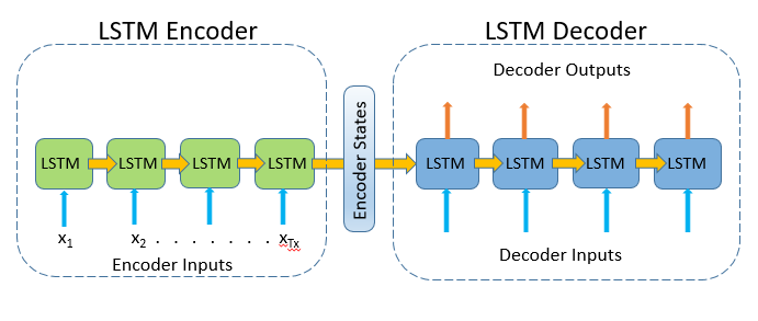
2.1.1 Breakdown
- The LSTM Encoder consists of 4 LSTM cells and the LSTM Decoder consists of 4 LSTM cells.
- Each input (word or word embedding) is fed into a new encoder LSTM cell together with the hidden state (output) from the previous LSTM cell
- The hidden state from the final LSTM encoder cell is (typically) the Encoder embedding. It can also be the entire sequence of hidden states from all encoder LSTM cells (note - this is not the same as attention)
- The LSTM decoder uses the encoder state(s) as input and procceses these iteratively through the various LSTM cells to produce the output. This can be unidirectional or bidirectional
Several extensions to the vanilla seq2seq model exists; the most notable being the Attention module.
Having discussed the seq2seq model, lets turn our attention to the task of frame prediction!
2.2 Frame Prediction
Frame prediction is inherently different from the original tasks of seq2seq such as machine translation. This is due to the fact, that RNN modules (LSTM) in the encoder and decoder use fully-connected layers to encode and decode word embeddings (which are represented as vectors).
Once we are dealing with frames we have 2D tensors, and to encode and decode these in a sequential nature we need an extension of the original LSTM seq2seq models.
2.2.1 ConvLSTM
This is where Convolutional LSTM (ConvLSTM) comes in. Presented at NIPS in 2015, ConvLSTM modifies the inner workings of the LSTM mechanism to use the convolution operation instead of simple matrix multiplication. Lets write our new equations for the ConvLSTM cells:
\begin{equation}i_{t}=\sigma\left(W_{x i} * X_{t}+W_{h i} * H_{t-1}+W_{c i} \circ C_{t-1}+b_{i}\right)\end{equation} \begin{equation}f_{t}=\sigma\left(W_{x f} * X_{t}+W_{h f} * H_{t-1}+W_{c f} \circ C_{t-1}+b_{f}\right)\end{equation} \begin{equation}C_{t}=f_{t} \circ C_{t-1}+i_{t} \circ \tanh \left(W_{x c} * X_{t}+W_{h c} * H_{t-1}+b_{c}\right)\end{equation} \begin{equation}o_{t}=\sigma\left(W_{x o} * X_{t}+W_{h o} * H_{t-1}+W_{c o} \circ C_{t}+b_{o}\right)\end{equation} \begin{equation}H_{t}=o_{t} \circ \tanh \left(C_{t}\right)\end{equation}
$*$ denotes the convolution operation and $\circ$ denotes the Hadamard product like before.
Can you spot the subtle difference between these equations and regular LSTM? We simply replace the multiplications in the four gates between
a) weight matrices and input ($W_{x} x_{t}$ with $W_{x} * X_{t}$) and
b) weight matrices and previous hidden state ($W_{h} h_{t-1}$ with $W_{h} * H_{t-1}$).
Otherwise, everything remains the same.
If you prefer not to dive into the above equations, the primary thing to note is the fact that we use convolutions (kernel) to process our input images to derive feature maps rather than vectors derived from fully-connected layers.
2.2.2 n-step Ahead Prediction
One of the most difficult things when designing frame prediction models (with ConvLSTM) is defining how to produce the frame predictions. We list two methods here (but others do also exist):
- Predict the next frame and feed it back into the network for a number of n steps to produce n frame predictions.
- Predict all future time steps in one-go by having the number of ConvLSTM layers l be equal to the number of n steps. Thus, we can simply use the output from each decoder LSTM cell as our predictions
In this tutorial we will focus on number 1 - especially since it can produce any number of predictions in the future without having to change the architecture completely. Furthermore, if we are to predict many steps in the future option 2 becomes increasingly computationally expensive.
2.2.3 ConvLSTM implementation
For our ConvLSTM implementation we use the pytorch implementation from ndrplz
It looks as follows:
import torch.nn as nn
import torch


class ConvLSTMCell(nn.Module):

    def __init__(self, input_dim, hidden_dim, kernel_size, bias):
        """
        Initialize ConvLSTM cell.

        Parameters
        ----------
        input_dim: int
            Number of channels of input tensor.
        hidden_dim: int
            Number of channels of hidden state.
        kernel_size: (int, int)
            Size of the convolutional kernel.
        bias: bool
            Whether or not to add the bias.
        """

        super(ConvLSTMCell, self).__init__()

        self.input_dim = input_dim
        self.hidden_dim = hidden_dim

        self.kernel_size = kernel_size
        self.padding = kernel_size[0] // 2, kernel_size[1] // 2
        self.bias = bias

        self.conv = nn.Conv2d(in_channels=self.input_dim + self.hidden_dim,
                              out_channels=4 * self.hidden_dim,
                              kernel_size=self.kernel_size,
                              padding=self.padding,
                              bias=self.bias)

    def forward(self, input_tensor, cur_state):
        h_cur, c_cur = cur_state

        combined = torch.cat([input_tensor, h_cur], dim=1)  # concatenate along channel axis

        combined_conv = self.conv(combined)
        cc_i, cc_f, cc_o, cc_g = torch.split(combined_conv, self.hidden_dim, dim=1)
        i = torch.sigmoid(cc_i)
        f = torch.sigmoid(cc_f)
        o = torch.sigmoid(cc_o)
        g = torch.tanh(cc_g)

        c_next = f * c_cur + i * g
        h_next = o * torch.tanh(c_next)

        return h_next, c_next

    def init_hidden(self, batch_size, image_size):
        height, width = image_size
        return (torch.zeros(batch_size, self.hidden_dim, height, width, device=self.conv.weight.device),
                torch.zeros(batch_size, self.hidden_dim, height, width, device=self.conv.weight.device))
Hopefully you can see how the equations defined earlier are written in the above code for the forward pass.
2.2.4 Seq2Seq implementation
The specific architecture we use looks as follows:
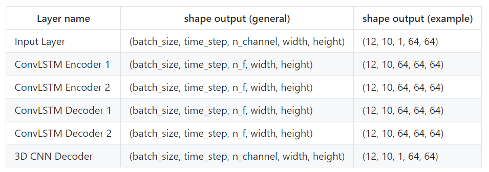
Encoder and Decoder
We use two ConvLSTM cells for both the encoder and the decoder (encoder_1_convlstm, encoder_2_convlstm, decoder_1_convlstm, decoder_2_convlstm).
3D CNN
Our final ConvLSTM cell (decoder_2convlstm) outputs _nf feature maps for each predicted frame (12, 10, 64, 64, 64).
As we are essentially doing regression (predicting pixel values), we need to transform these feature maps into actual predictions similar to what you do in classical image classification.
To achieve this we implement a 3D-CNN layer. The 3D CNN layer does the following: 1) Takes as input (nf, width, height) for each batch and time_step 2) Iterates over all n predicted frames using 3D kernel 3) Outputs one channel (1, width, height) per image - i.e., the predicted pixel values
Sigmoid layer
Finally, as we have transformed the pixel values into [0, 1] we use a sigmoid function to turn our 3D CNN activations into [0, 1].
And that is basically it!
Now we define the python implementation for the seq2seq model:
import torch
import torch.nn as nn

from models.ConvLSTMCell import ConvLSTMCell

class EncoderDecoderConvLSTM(nn.Module):
    def __init__(self, nf, in_chan):
        super(EncoderDecoderConvLSTM, self).__init__()

        """ ARCHITECTURE

        # Encoder (ConvLSTM)
        # Encoder Vector (final hidden state of encoder)
        # Decoder (ConvLSTM) - takes Encoder Vector as input
        # Decoder (3D CNN) - produces regression predictions for our model

        """
        self.encoder_1_convlstm = ConvLSTMCell(input_dim=in_chan,
                                               hidden_dim=nf,
                                               kernel_size=(3, 3),
                                               bias=True)

        self.encoder_2_convlstm = ConvLSTMCell(input_dim=nf,
                                               hidden_dim=nf,
                                               kernel_size=(3, 3),
                                               bias=True)

        self.decoder_1_convlstm = ConvLSTMCell(input_dim=nf,  # nf + 1
                                               hidden_dim=nf,
                                               kernel_size=(3, 3),
                                               bias=True)

        self.decoder_2_convlstm = ConvLSTMCell(input_dim=nf,
                                               hidden_dim=nf,
                                               kernel_size=(3, 3),
                                               bias=True)

        self.decoder_CNN = nn.Conv3d(in_channels=nf,
                                     out_channels=1,
                                     kernel_size=(1, 3, 3),
                                     padding=(0, 1, 1))


    def autoencoder(self, x, seq_len, future_step, h_t, c_t, h_t2, c_t2, h_t3, c_t3, h_t4, c_t4):

        outputs = []

        # encoder
        for t in range(seq_len):
            h_t, c_t = self.encoder_1_convlstm(input_tensor=x[:, t, :, :],
                                               cur_state=[h_t, c_t])  # we could concat to provide skip conn here
            h_t2, c_t2 = self.encoder_2_convlstm(input_tensor=h_t,
                                                 cur_state=[h_t2, c_t2])  # we could concat to provide skip conn here

        # encoder_vector
        encoder_vector = h_t2

        # decoder
        for t in range(future_step):
            h_t3, c_t3 = self.decoder_1_convlstm(input_tensor=encoder_vector,
                                                 cur_state=[h_t3, c_t3])  # we could concat to provide skip conn here
            h_t4, c_t4 = self.decoder_2_convlstm(input_tensor=h_t3,
                                                 cur_state=[h_t4, c_t4])  # we could concat to provide skip conn here
            encoder_vector = h_t4
            outputs += [h_t4]  # predictions

        outputs = torch.stack(outputs, 1)
        outputs = outputs.permute(0, 2, 1, 3, 4)
        outputs = self.decoder_CNN(outputs)
        outputs = torch.nn.Sigmoid()(outputs)

        return outputs

    def forward(self, x, future_seq=0, hidden_state=None):

        """
        Parameters
        ----------
        input_tensor:
            5-D Tensor of shape (b, t, c, h, w)        #   batch, time, channel, height, width
        """

        # find size of different input dimensions
        b, seq_len, _, h, w = x.size()

        # initialize hidden states
        h_t, c_t = self.encoder_1_convlstm.init_hidden(batch_size=b, image_size=(h, w))
        h_t2, c_t2 = self.encoder_2_convlstm.init_hidden(batch_size=b, image_size=(h, w))
        h_t3, c_t3 = self.decoder_1_convlstm.init_hidden(batch_size=b, image_size=(h, w))
        h_t4, c_t4 = self.decoder_2_convlstm.init_hidden(batch_size=b, image_size=(h, w))

        # autoencoder forward
        outputs = self.autoencoder(x, seq_len, future_seq, h_t, c_t, h_t2, c_t2, h_t3, c_t3, h_t4, c_t4)

        return outputs
3. Training
Maybe you are already aware of the excellent library pytorch-lightning, which essentially takes all the boiler-plate engineering out of machine learning when using pytorch, such as the following commands: optimizer.zero_grad(), optimizer.step().
It also standardizes training modules and enables easy multi-GPU functionality and mixed-precision training for Volta architecture GPU cards.
There is so much functionality available in pytorch-lightning, and I will try to demonstrate the workflow I have created, which I think works fairly well.
# import libraries
import os
import matplotlib.pyplot as plt
import torch
import torchvision
from torch.nn import functional as F
from torch.utils.data import DataLoader
import pytorch_lightning as pl
from pytorch_lightning import Trainer
from multiprocessing import Process

from utils.start_tensorboard import run_tensorboard
from models.seq2seq_ConvLSTM import EncoderDecoderConvLSTM
from data.MovingMNIST import MovingMNIST

import argparse

parser = argparse.ArgumentParser()
parser.add_argument('--lr', default=1e-4, type=float, help='learning rate')
parser.add_argument('--beta_1', type=float, default=0.9, help='decay rate 1')
parser.add_argument('--beta_2', type=float, default=0.98, help='decay rate 2')
parser.add_argument('--batch_size', default=12, type=int, help='batch size')
parser.add_argument('--epochs', type=int, default=300, help='number of epochs to train for')
parser.add_argument('--use_amp', default=False, type=bool, help='mixed-precision training')
parser.add_argument('--n_gpus', type=int, default=1, help='number of GPUs')
parser.add_argument('--n_hidden_dim', type=int, default=64, help='number of hidden dim for ConvLSTM layers')

opt = parser.parse_args()

##########################
######### MODEL ##########
##########################

class MovingMNISTLightning(pl.LightningModule):

    def __init__(self, hparams=None, model=None):
        super(MovingMNISTLightning, self).__init__()

        # default config
        self.path = os.getcwd() + '/data'
        self.normalize = False
        self.model = model

        # logging config
        self.log_images = True

        # Training config
        self.criterion = torch.nn.MSELoss()
        self.batch_size = opt.batch_size
        self.n_steps_past = 10
        self.n_steps_ahead = 10  # 4

    def create_video(self, x, y_hat, y):
        # predictions with input for illustration purposes
        preds = torch.cat([x.cpu(), y_hat.unsqueeze(2).cpu()], dim=1)[0]

        # entire input and ground truth
        y_plot = torch.cat([x.cpu(), y.unsqueeze(2).cpu()], dim=1)[0]

        # error (l2 norm) plot between pred and ground truth
        difference = (torch.pow(y_hat[0] - y[0], 2)).detach().cpu()
        zeros = torch.zeros(difference.shape)
        difference_plot = torch.cat([zeros.cpu().unsqueeze(0), difference.unsqueeze(0).cpu()], dim=1)[
            0].unsqueeze(1)

        # concat all images
        final_image = torch.cat([preds, y_plot, difference_plot], dim=0)

        # make them into a single grid image file
        grid = torchvision.utils.make_grid(final_image, nrow=self.n_steps_past + self.n_steps_ahead)

        return grid

    def forward(self, x):
        x = x.to(device='cuda')

        output = self.model(x, future_seq=self.n_steps_ahead)

        return output

    def training_step(self, batch, batch_idx):
        x, y = batch[:, 0:self.n_steps_past, :, :, :], batch[:, self.n_steps_past:, :, :, :]
        x = x.permute(0, 1, 4, 2, 3)
        y = y.squeeze()

        y_hat = self.forward(x).squeeze()  # is squeeze neccessary?

        loss = self.criterion(y_hat, y)

        # save learning_rate
        lr_saved = self.trainer.optimizers[0].param_groups[-1]['lr']
        lr_saved = torch.scalar_tensor(lr_saved).cuda()

        # save predicted images every 250 global_step
        if self.log_images:
            if self.global_step % 250 == 0:
                final_image = self.create_video(x, y_hat, y)

                self.logger.experiment.add_image(
                    'epoch_' + str(self.current_epoch) + '_step' + str(self.global_step) + '_generated_images',
                    final_image, 0)
                plt.close()

        tensorboard_logs = {'train_mse_loss': loss,
                            'learning_rate': lr_saved}

        return {'loss': loss, 'log': tensorboard_logs}


    def test_step(self, batch, batch_idx):
        # OPTIONAL
        x, y = batch
        y_hat = self.forward(x)
        return {'test_loss': self.criterion(y_hat, y)}


    def test_end(self, outputs):
        # OPTIONAL
        avg_loss = torch.stack([x['test_loss'] for x in outputs]).mean()
        tensorboard_logs = {'test_loss': avg_loss}
        return {'avg_test_loss': avg_loss, 'log': tensorboard_logs}


    def configure_optimizers(self):
        return torch.optim.Adam(self.parameters(), lr=opt.lr, betas=(opt.beta_1, opt.beta_2))

    @pl.data_loader
    def train_dataloader(self):
        train_data = MovingMNIST(
            train=True,
            data_root=self.path,
            seq_len=self.n_steps_past + self.n_steps_ahead,
            image_size=64,
            deterministic=True,
            num_digits=2)

        train_loader = torch.utils.data.DataLoader(
            dataset=train_data,
            batch_size=self.batch_size,
            shuffle=True)

        return train_loader

    @pl.data_loader
    def test_dataloader(self):
        test_data = MovingMNIST(
            train=False,
            data_root=self.path,
            seq_len=self.n_steps_past + self.n_steps_ahead,
            image_size=64,
            deterministic=True,
            num_digits=2)

        test_loader = torch.utils.data.DataLoader(
            dataset=test_data,
            batch_size=self.batch_size,
            shuffle=True)

        return test_loader


def run_trainer():
    conv_lstm_model = EncoderDecoderConvLSTM(nf=opt.n_hidden_dim, in_chan=1)

    model = MovingMNISTLightning(model=conv_lstm_model)

    trainer = Trainer(max_epochs=opt.epochs,
                      gpus=opt.n_gpus,
                      distributed_backend='dp',
                      early_stop_callback=False,
                      use_amp=opt.use_amp
                      )

    trainer.fit(model)


if __name__ == '__main__':
    p1 = Process(target=run_trainer)                    # start trainer
    p1.start()
    p2 = Process(target=run_tensorboard(new_run=True))  # start tensorboard
    p2.start()
    p1.join()
    p2.join()
Most of the functionality of class MovingMNISTLightning is fairly self-explanatory. Here is the overall workflow:
1) We instantiate our class and define all the relevant parameters 2) We take a training_step (for each batch), where we – a) create a prediction y_hat – b) calculate the MSE loss – c) save a visualization of the prediction with input and ground truth every 250 global step into tensorboard – d) save the learning rate and loss for each batch into tensorboard
When we actually run our main.py script we can define several relevant parameters. For example, if we want to run with 2 GPUs, mixed-precision and batch_size = 16 we simply type:
python main.py --n_gpus=2 --use_amp=True --batch_size=16
Feel free to experiment with various configurations!
When we run the main.py script we automatically spin up a tensorboard session using multiprocessing, and here you can track the performance of our model iteratively and also see the visualization of our predictions every 250 global step.